728x90
사이킷런 제공 임곗값 변화에 따른 평가지표 API
precision_recall_curve()
from sklearn.metrics import precision_recall_curve#앞인덱스0 , 뒤인덱스 1인거 가져옴
#레이블값 1일때 예측확률값 pred_proba()의 반환 ndarray 두번째 칼럼(칼럼인덱스 1)
pred_proba[:,1]##실제값 데이터세트와 위 값(레이블값1일때 예측확률
precision_recall_curve(y_test,pred_proba[:,1])
#실제값 데이터세트, 예측확률
def precision_recall_curve_plot(y_test,pred_proba):
    #thresholds에 따른 정밀도, 재현율 추출
    precisions,recalls,thresholds = precision_recall_curve(y_test,
                                                          pred_proba)
    plt.figure(figsize=(8,6))
    ##행렬값 반환
    threshold_boundary = thresholds.shape[0]
    #x축에 threshold값 ,y축 예측값(0부터 threshold_boundary까지)
    #y축은 정밀도, 재현율 값으로 두개 선 그려줌 정밀도는 점선으로 표시
    plt.plot(thresholds,
             precisions[0:threshold_boundary],
             linestyle='--',
             label='precision')
    #y축은 recall값
    plt.plot(thresholds,
             recalls[0:threshold_boundary],
             label='recall')
    #x축값을 시작값 끝값으로 설정
    start,end = plt.xlim()
    #threshold 값 x축 간격 0.1로 변경
    plt.xticks(np.round(np.arange(start,end,0.1),2))
    #레이블값
    plt.legend()
    #눈금있는 위치에 줄그음
    plt.grid()
    plt.show()

#두번째열 (인덱스 1)
precision_recall_curve_plot(y_test,pred_proba[:,1])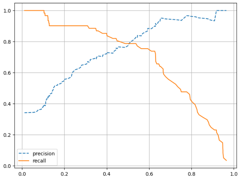
F1 스코어
get_eval_by_threshold() 함수 이용해 임계값 0.4~0.6 별로 정확도 ,정밀도, 재현율, F1 스코어
#pred_prob=None 기본값 상황에 따라 안들어올수있음
def get_clf_eval(y_test,pred=None,pred_proba=None):
    ##평가모델은 metrics 에 있음
    ##confusion_matrix 오차행렬 precision_score 정밀도 ,recall_score 재현율
    ##accuracy_score 정확도 ,f1스코어 추가
    from sklearn.metrics import accuracy_score,confusion_matrix,precision_score,recall_score,f1_score,roc_auc_score
    confusion = confusion_matrix(y_test,pred)
    accuracy = accuracy_score(y_test,pred)
    precision = precision_score(y_test,pred)
    recall = recall_score(y_test,pred)
    f1 = f1_score(y_test,pred)
    ##roc 추가
    roc_auc = roc_auc_score(y_test,pred_proba)

    print('오차행렬')
    print(confusion)
    print(f'정확도:{accuracy:.4f},정밀도:{precision:.4f},재현율:{recall:.4f},f1:{f1:.4f},AUC:{roc_auc:.4f}')

#실제값,
def get_eval_by_threshold(y_test,pred_proba,thresholds):
    #thresholds 개수만큼 한개씩 뽑아옴 ex)0.4 ...
    from sklearn.preprocessing import Binarizer
    for threshold in thresholds:
        pred = Binarizer(threshold=threshold).fit_transform(pred_proba)
        print('임계값:', threshold)
        get_clf_eval(y_test,pred)
thresholds = [0.4,0.45,0.5,0.55,0.6]
#첫번째 열
#.reshape(-1,1) 오류나서 추가한 부분
pred_proba = lr_clf.predict_proba(x_test)[:,1].reshape(-1,1)
#pred_proba.reshape(-1,1)로 써도 위와 같음
get_eval_by_threshold(y_test,pred_proba,thresholds)결과
임계값: 0.4
오차행렬
[[98 20]
 [10 51]]
정확도:0.8324,정밀도:0.7183,재현율:0.8361,f1:0.7727
임계값: 0.45
오차행렬
[[103  15]
 [ 12  49]]
정확도:0.8492,정밀도:0.7656,재현율:0.8033,f1:0.7840
임계값: 0.5
오차행렬
[[104  14]
 [ 13  48]]
정확도:0.8492,정밀도:0.7742,재현율:0.7869,f1:0.7805
임계값: 0.55
오차행렬
[[109   9]
 [ 15  46]]
정확도:0.8659,정밀도:0.8364,재현율:0.7541,f1:0.7931
임계값: 0.6
오차행렬
[[112   6]
 [ 16  45]]
정확도:0.8771,정밀도:0.8824,재현율:0.7377,f1:0.8036
f1스코어는 임계값이 0.6일때 가장 좋은
재현율이 크게 감소
오류
Reshape your data either using array.reshape(-1, 1) if your data has a single feature or array.reshape(1, -1) if it contains a single sample.해결
pred_proba = lr_clf.predict_proba(x_test)[:,1].reshape(-1,1) 로 수정
뒤에 reshape 으로 수정
ROC 곡선과 AUC
예측성능 판단 지표
ROC곡선 : FPR이 변할때 TPR변화를 나타내는 곡선
FPR(False Positive Rate) - X축
- > TP / (FN + TP) 재현율(민감도)
민감도에 대응하는 지표인 TNR(True Negative Rage)특이성
TPR(True Positive Rate) - Y축
FPR을 0 부터 1까지 변경하면서 TPR의 변화 값 구함
어떻게 변경? 분류결정 임계값을 변경한다.
ROC곡선 구하는 roc_curve() api 사용
def roc_curve_plot(y_test,pred_prob):
    fprs,tprs,thresholds = roc_curve(y_test,pred_prob)
    ##y_test: 실제값 array , y_score :pred_proba의 반환값
    plt.plot(fprs,tprs,label='ROC')
    plt.plot([0,1],[0,1],'k--',label='Random')
    start,end = plt.xlim()
    #x축 단위를 0.1로 변경
    plt.xticks(np.round(np.arange(start,end,0.1) ,2))
    plt.xlim(0,1)
    plt.ylim(0,1)
    #레이블표시
    plt.legend()
    plt.show()

roc_curve_plot(y_test,pred_proba)
피마인디언 당뇨병 예측
import numpy as np
import pandas as pd
import matplotlib.pyplot as plt

from sklearn.model_selection import train_test_split
from sklearn.preprocessing import StandardScaler
from sklearn.linear_model import LogisticRegression

df = pd.read_csv("diabetes.csv")
앙상블 방법
정보 균일도 측정 방법 : 엔트로피를 이용한 정보이득
정보이득지수 = 1 - 엔트로피지수
높은게 균일도 높음
지니계수 : 0 이 가장 평등, 1로 갈수록 불평등
지니계수 낮을 수록 균일도 높음
728x90
